💡 학습 팁: 통계 수식과 용어가 낯설고 어렵다면? 아주 쉽게 풀어쓴 📖 쉬운 해설(의역본) 보기를 추천합니다!

2.2.3 The Classification Setting_

2.2.3 분류 설정_

Thus far, our discussion of model accuracy has been focused on the regression setting.

지금까지, 모형 정확도에 대한 우리의 논의는 회귀 설정에 집중되어 왔습니다.

But many of the concepts that we have encountered, such as the bias-variance trade-off, transfer over to the classification setting with only some modifications due to the fact that $y_i$ is no longer quantitative.

하지만 편향-분산 트레이드오프와 같이 우리가 접했던 많은 개념들은 $y_i$ 가 더 이상 양적이지 않다는 사실로 인한 약간의 수정들만을 지닌 채 분류 설정으로 넘어갑니다.

Suppose that we seek to estimate $f$ on the basis of training observations ${(x_1, y_1), \dots , (x_n, y_n)}$, where now $y_1, \dots , y_n$ are qualitative.

우리가 이제 $y_1, \dots , y_n$ 이 질적인 훈련 관측치들 ${(x_1, y_1), \dots , (x_n, y_n)}$ 에 기초하여 $f$ 를 추정하려고 시도한다고 가정해 보십시오.

The most common approach for quantifying the accuracy of our estimate $\hat{f}$ is the training error rate , the proportion of mistakes that are made if we apply our estimate $\hat{f}$ to the training observations:

우리의 추정치 $\hat{f}$ 의 정확도를 정량화하기 위한 가장 흔한 접근법은 훈련 오차율(error rate) 이며, 이것은 우리가 훈련 관측치들에 우리의 추정치 $\hat{f}$ 를 적용할 때 만들어지는 실수들의 비율입니다:

\[\frac{1}{n} \sum_{i=1}^n I(y_i \neq \hat{y}_i) \tag{2.8}\]

Here $\hat{y}_i$ is the predicted class label for the $i$th observation using $\hat{f}$.

여기서 $\hat{y}_i$ 는 $\hat{f}$ 를 사용한 $i$번째 관측치에 대한 예측된 클래스 라벨입니다.

And $I(y_i \neq \hat{y}i)$ is an _indicator variable that equals 1 if $y_i \neq \hat{y}_i$ and zero if $y_i = \hat{y}_i$.

그리고 $I(y_i \neq \hat{y}i)$ 는 만약 $y_i \neq \hat{y}_i$ 라면 1과 같고 만약 $y_i = \hat{y}_i$ 라면 0과 같은 _지시 변수(indicator variable) 입니다.

If $I(y_i \neq \hat{y}_i) = 0$ then the $i$th observation was classified correctly by our classification method; otherwise it was misclassified.

만약 $I(y_i \neq \hat{y}_i) = 0$ 이라면 $i$번째 관측치는 우리의 분류 방법에 의해 올바르게 분류되었습니다; 그렇지 않다면 그것은 오분류되었습니다.

Hence Equation 2.8 computes the fraction of incorrect classifications.

그러므로 방정식 2.8은 올바르지 않은 분류들의 비율을 계산합니다.

Equation 2.8 is referred to as the training error rate because it is computed based on the data that was used to train our classifier.

방정식 2.8은 우리의 분류기를 훈련시키는 데 사용되었던 데이터에 기초하여 계산되기 때문에 훈련 오차율(training error rate) 로 지칭되어집니다.

As in the regression setting, we are most interested in the error rates that result from applying our classifier to test observations that were not used in training.

회귀 설정에서와 같이, 우리는 훈련에 사용되지 않은 시험 관측치들에 우리의 분류기를 적용하는 것으로부터 도출되는 오차율들에 가장 관심이 있습니다.

The test error rate associated with a set of test observations of the form $(x_0, y_0)$ is given by

형태 $(x_0, y_0)$ 의 시험 관측치들의 집합과 연관된 시험 오차율(test error rate) 은 다음과 같이 주어집니다

\[\text{Ave}(I(y_0 \neq \hat{y}_0)) \tag{2.9}\]

where $\hat{y}_0$ is the predicted class label that results from applying the classifier to the test observation with predictor $x_0$.

여기서 $\hat{y}_0$ 는 예측 변수 $x_0$ 와 함께 시험 관측치에 분류기를 적용하는 것으로부터 산출되는 예측된 클래스 라벨입니다.

A good classifier is one for which the test error (2.9) is smallest.

좋은(good) 분류기란 시험 오차 (2.9)가 가장 작은 것을 의미합니다.

The Bayes Classifier

베이즈 분류기

It is possible to show (though the proof is outside of the scope of this book) that the test error rate given in (2.9) is minimized, on average, by a very simple classifier that assigns each observation to the most likely class, given its predictor values .

(비록 증명은 이 책의 범위를 벗어나지만) (2.9)에 주어진 시험 오차율은 평균적으로, 자신의 예측 변수 값들이 주어졌을 때 각각의 관측치를 가장 가능성 있는 클래스에 할당하는 매우 단순한 분류기에 의해 최소화된다는 것을 보여 주는 것이 가능합니다.

In other words, we should simply assign a test observation with predictor vector $x_0$ to the class $j$ for which

다시 말해서, 우리는 예측 변수 벡터 $x_0$ 를 가진 시험 관측치를 다음 식 값이 가장 큰 클래스 $j$ 에 단순히 할당해야만 합니다

\[Pr(Y = j|X = x_0) \tag{2.10}\]

Note that (2.10) is a conditional probability : it is the probability that $Y = j$, given the observed predictor vector $x_0$.

(2.10)은 조건부 확률(conditional probability) 임을 주목하십시오: 이는 관측된 예측 변수 벡터 $x_0$ 가 주어질 때 $Y = j$ 일 확률입니다.

This very simple classifier is called the Bayes classifier .

이 매우 단순한 분류기는 베이즈 분류기(Bayes classifier) 로 불려집니다.

In a two-class problem where there are only two possible response values, say class 1 or class 2 , the Bayes classifier corresponds to predicting class one if $Pr(Y = 1

X = x_0) > 0.5$, and class two otherwise.

오직 두 가지의 가능한 응답 값들, 예를 들어 클래스 1 또는 클래스 2 만 있는 두-클래스 문제에서, 베이즈 분류기는 만약 $Pr(Y = 1

X = x_0) > 0.5$ 이면 클래스 1을 예측하는 것에, 그렇지 않다면 클래스 2를 예측하는 것에 해당합니다.

Figure 2.13 provides an example using a simulated data set in a two-dimensional space consisting of predictors $X_1$ and $X_2$.

그림 2.13은 예측 변수들 $X_1$ 과 $X_2$ 로 구성된 2차원 공간 안의 시뮬레이션된 데이터 세트를 사용하는 예를 제공합니다.

The orange and blue circles correspond to training observations that belong to two different classes.

주황색과 파란색 원들은 서로 다른 두 가지 클래스들에 속하는 훈련 관측치들에 해당합니다.

For each value of $X_1$ and $X_2$, there is a different probability of the response being orange or blue.

$X_1$ 과 $X_2$ 의 각각의 값에 대하여, 응답이 주황색 또는 파란색이 될 서로 다른 확률이 존재합니다.

Since this is simulated data, we know how the data were generated and we can calculate the conditional probabilities for each value of $X_1$ and $X_2$.

이것은 시뮬레이션된 데이터이기 때문에, 우리는 데이터가 어떻게 생성되었는지를 알고 있으며 우리는 $X_1$ 과 $X_2$ 의 각각의 값에 대하여 조건부 확률들을 계산할 수 있습니다.

The orange shaded region reflects the set of points for which $Pr(Y = \text{orange}

X)$ is greater than 50 %, while the blue shaded region indicates the set of points for which the probability is below 50 %.

주황색으로 음영 처리된 영역은 $Pr(Y = \text{orange}

X)$ 가 50%를 상회하는 점들의 집합을 반영하는 반면, 파란색으로 음영 처리된 영역은 그 확률이 50%의 미만인 점들의 집합을 기리킵니다.

The purple dashed line represents the points where the probability is exactly 50 %.

보라색 점선은 그 확률이 정확히 50%가 되는 점들을 상징하여 나타냅니다.

This is called the Bayes decision boundary .

이것은 베이즈 결정 경계(Bayes decision boundary) 제반으로 불려집니다.

The Bayes classifier’s prediction is determined by the Bayes decision boundary; an observation that falls on the orange side of the boundary will be assigned to the orange class, and similarly an observation on the blue side of the boundary will be assigned to the blue class.

베이즈 분류기의 예측은 베이즈 결정 경계에 의해 결정됩니다; 경계의 주황색 측면에 떨어지는 관측치는 주황색 클래스에 할당될 것이고, 유사하게 경계의 파란색 측면에 떨어지는 관측치는 파란색 클래스에 할당될 것입니다.

Figure 2.13

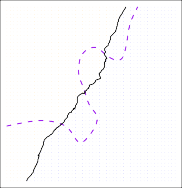
FIGURE 2.13. A simulated data set consisting of 100 observations in each of two groups, indicated in blue and in orange. The purple dashed line represents the Bayes decision boundary. The orange background grid indicates the region in which a test observation will be assigned to the orange class, and the blue background grid indicates the region in which a test observation will be assigned to the blue class.

그림 2.13. 파란색과 주황색으로 표시된 두 그룹들 각각 안에서 100개의 관측치들로 구성된 시뮬레이션된 데이터 세트. 보라색 점선은 베이즈 결정 경계를 나타냅니다. 주황색 배경 격자는 시험 관측치가 주황색 클래스로 할당될 영역을 가리키고, 파란색 배경 격자는 시험 관측치가 파란색 클래스로 할당될 영역을 가리킵니다.

The Bayes classifier produces the lowest possible test error rate, called the Bayes error rate.

베이즈 분류기는 베이즈 오차율(Bayes error rate) 로 불리는 가장 낮은 발생 가능한 시험 오차율을 산출합니다.

Since the Bayes classifier will always choose the class for which (2.10) is largest, the error rate will be $1 - \max_j Pr(Y=j

X=x_0)$ at $X=x_0$.

베이즈 분류기는 항상 (2.10)이 가장 커지는 클래스를 선택할 것이기 때문에, 그 오차율은 $X=x_0$ 에서 $1 - \max_j Pr(Y=j

X=x_0)$ 이 될 것입니다.

In general, the overall Bayes error rate is given by

일반적으로, 종합적인 통계상의 베이즈 오차율 공식은 다음과 같이 주어집니다

\[1 - E(\max_j Pr(Y=j|X)) \tag{2.11}\]

where the expectation averages the probability over all possible values of $X$ .

여기서 기댓값은 $X$ 의 모든 가능한 수치 값들에 걸쳐 확률을 일괄 평균 치수화 합니다.

For our simulated data, the Bayes error rate is 0.133.

우리의 시뮬레이션된 데이터에 대하여, 이 베이즈 오차율 수치는 0.133에 해당합니다.

It is greater than zero, because the classes overlap in the true population, which implies that $\max_j Pr(Y = j

X = x_0) < 1$ for some values of $x_0$.

해당 클래스 군집들이 진정한 대상 모집단 내부에서 겹쳐 분포하기 때문에 통계상 그것은 제로 0보다 항상 크며, 이는 $x_0$ 의 일부 측정된 값들에 대해 $\max_j Pr(Y = j

X = x_0) < 1$ 임을 필시 내포하여 가리킵니다.

The Bayes error rate is analogous to the irreducible error, discussed earlier.

결과적으로 이 베이즈 오차율 공식은 앞서 논의하여 다루었던 줄일 수 없는 오차와 유사합니다.

2.2.3.1 K-Nearest Neighbors (K-최근접 이웃)

비모수적인 분류 환경에서 이론의 실제 구현체로 가장 직관적인 알고리즘인 K-최근접 이웃(KNN) 기법을 학습합니다. K 값의 크기 변화에 따라 결정 경계(Decision Boundary)가 어떻게 바뀌며, 그 과정 속 편향-분산 트레이드오프가 나타나는지를 배웁니다.

Sub-Chapters (하위 목차)

< 2.2.2 The Bias-Variance Trade-Off

2.2.3.1 K Nearest Neighbors >

서브목차