| < 2. Statistical Learning | 2.1.1 Why Estimate F > |
💡 학습 팁: 원문 해석이 어렵다면? 한 줄씩 나란히 번역된 📖 직역본 보기를 추천합니다!
2.1 What Is Statistical Learning?
In order to motivate our study of statistical learning, we begin with a simple example.
Suppose that we are statistical consultants hired by a client to investigate the association between advertising and sales of a particular product. The Advertising data set consists of the sales of that product in 200 different markets, along with advertising budgets for the product in each of those markets for three different media: TV , radio , and newspaper . The data are displayed in Figure 2.1. It is not possible for our client to directly increase sales of the product.
On the other hand, they can control the advertising expenditure in each of the three media. Therefore, if we determine that there is an association between advertising and sales, then we can instruct our client to adjust advertising budgets, thereby indirectly increasing sales.
In other words, our goal is to develop an accurate model that can be used to predict sales on the basis of the three media budgets.
In this setting, the advertising budgets are input variables while sales is an output variable .
The input variables are typically denoted using the variable symbol X , with a subscript to distinguish them. So $X_1$ might be the TV budget, $X_2$ the radio budget, and $X_3$ the newspaper budget.
The input variables go by different names, such as predictors , independent variables , features , or sometimes just variables .
The output variable—in this case, sales —is often called the response or dependent variable , and is typically denoted using the symbol Y .
Throughout this book, we will use all of these terms interchangeably.
More generally, suppose that we observe a quantitative response Y and p different predictors, $X_1, X_2, . . . , X_p$.
We assume that there is some relationship between Y and $X = (X_1, X_2, . . . , X_p)$, which can be written in the very general form
\[Y = f(X) + \epsilon \tag{2.1}\]
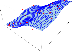
FIGURE 2.1. The Advertising data set. The plot displays sales , in thousands of units, as a function of TV , radio , and newspaper budgets, in thousands of dollars, for 200 different markets. In each plot we show the simple least squares fit of sales to that variable, as described in Chapter 3. In other words, each blue line represents a simple model that can be used to predict sales using TV , radio , and newspaper , respectively.
Here f is some fixed but unknown function of $X_1, . . . , X_p$ , and ϵ is a random error term , which is independent of X and has mean zero.
In this formulation, f represents the systematic information that X provides about Y .
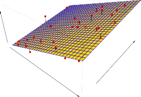
FIGURE 2.2. The Income data set. Left: The red dots are the observed values of income (in thousands of dollars) and years of education for 30 individuals. Right: The blue curve represents the true underlying relationship between income and years of education , which is generally unknown (but is known in this case because the data were simulated). The black lines represent the error associated with each observation. Note that some errors are positive (if an observation lies above the blue curve) and some are negative (if an observation lies below the curve). Overall, these errors have approximately mean zero.
As another example, consider the left-hand panel of Figure 2.2, a plot of income versus years of education for 30 individuals in the Income data set.
The plot suggests that one might be able to predict income using years of education.
However, the function f that connects the input variable to the output variable is in general unknown.
In this situation one must estimate f based on the observed points.
Since Income is a simulated data set, f is known and is shown by the blue curve in the right-hand panel of Figure 2.2. The vertical lines represent the error terms ϵ . We note that some of the 30 observations lie above the blue curve and some lie below it; overall, the errors have approximately mean zero.
In general, the function f may involve more than one input variable.
In Figure 2.3 we plot income as a function of years of education and seniority .
Here f is a two-dimensional surface that must be estimated based on the observed data.
In essence, statistical learning refers to a set of approaches for estimating f .
In this chapter we outline some of the key theoretical concepts that arise in estimating f , as well as tools for evaluating the estimates obtained.
2.1.1 Why Estimate f ?
Learn the prediction-centric reasons for predicting output values for new data points and the inference-centric reasons for analyzing the effect of each input variable on the output variable.
2.1.2 How Do We Estimate f ?
Introduces the approach to mathematically construct the most appropriate function $f$ utilizing Training Data. Covers the fundamental differences and theoretical workings of Parametric and Non-Parametric models.
2.1.3 The Trade-Off Between Prediction Accuracy and Model Interpretability
Addresses the black-box structure phenomenon where as a model becomes more flexible and powerful, its internal structure becomes more complex. Cultivates the ability to determine the level of flexibility based on the core purpose of the analysis.
2.1.4 Supervised Versus Unsupervised Learning
Examines the difference between supervised learning in environments where a label/response to be predicted is given, and unsupervised learning which only identifies structural characteristics.
2.1.5 Regression Versus Classification Problems
Defines a regression situation where the response variable is numerically continuous, and a classification situation where it is divided qualitatively into discrete classes.
Sub-Chapters
| < 2. Statistical Learning | 2.1.1 Why Estimate F > |