| < 2. Statistical Learning | 2.1.1 Why Estimate F > |
💡 학습 팁: 통계 수식과 용어가 낯설고 어렵다면? 아주 쉽게 풀어쓴 📖 쉬운 해설(의역본) 보기를 추천합니다!
2.1 What Is Statistical Learning?
2.1 통계적 학습이란 무엇인가?
In order to motivate our study of statistical learning, we begin with a simple example.
통계적 학습에 대한 우리의 연구 동기를 부여하기 위해 간단한 예제부터 시작합니다.
Suppose that we are statistical consultants hired by a client to investigate the association between advertising and sales of a particular product.
우리가 특정 제품의 광고와 판매 간의 연관성을 조사하기 위해 클라이언트가 고용한 통계 컨설턴트라고 가정해 보십시오.
The Advertising data set consists of the sales of that product in 200 different markets, along with advertising budgets for the product in each of those markets for three different media: TV , radio , and newspaper .
Advertising 데이터 세트는 200개의 서로 다른 시장에서의 해당 제품 판매량(sales)과, 그 시장들 각각의 세 가지 다른 매체: TV, radio, 그리고 newspaper 에 대한 해당 제품의 광고 예산들로 구성됩니다.
The data are displayed in Figure 2.1.
그 데이터는 그림 2.1에 표시되어 있습니다.
It is not possible for our client to directly increase sales of the product.
클라이언트가 제품의 판매를 직접적으로 늘리는 것은 불가능합니다.
On the other hand, they can control the advertising expenditure in each of the three media.
반면에 그들은 세 미디어 각각에서의 광고 지출을 통제할 수 있습니다.
Therefore, if we determine that there is an association between advertising and sales, then we can instruct our client to adjust advertising budgets, thereby indirectly increasing sales.
따라서, 만약 우리가 광고와 판매 사이에 연관성이 있다고 결정한다면, 우리는 클라이언트에게 광고 예산들을 조정하도록 지시하여 간접적으로 판매를 증가시킬 수 있습니다.
In other words, our goal is to develop an accurate model that can be used to predict sales on the basis of the three media budgets.
다시 말해서, 우리의 목표는 세 미디어 예산들에 기초하여 판매를 예측하는 데 쓰일 수 있는 정확한 모델을 개발하는 것입니다.
In this setting, the advertising budgets are input variables while sales is an output variable .
이러한 설정에서 광고 예산은 입력 변수들(input variables) 인 반면 sales 는 출력 변수(output variable) 입니다.
The input variables are typically denoted using the variable symbol X , with a subscript to distinguish them.
입력 변수들은 그것들을 구별하기 위한 아래첨자와 함께 대체로 변수 기호 X 를 사용하여 표기됩니다.
So $X_1$ might be the TV budget, $X_2$ the radio budget, and $X_3$ the newspaper budget.
따라서 $X_1$ 은 TV 예산, $X_2$ 는 radio 예산, 그리고 $X_3$ 는 newspaper 예산일 수 있습니다.
The input variables go by different names, such as predictors , independent variables , features , or sometimes just variables .
입력 변수들은 예측 변수들(predictors), 독립 변수들(independent variables), 특징들(features), 또는 때로는 그저 변수들(variables) 과 같은 여러가지 이름들로 불립니다.
The output variable—in this case, sales —is often called the response or dependent variable , and is typically denoted using the symbol Y .
출력 변수—이 경우 sales—는 종종 응답(response) 이나 종속 변수(dependent variable) 로 불리며, 일반적으로 기호 Y 를 사용하여 표시됩니다.
Throughout this book, we will use all of these terms interchangeably.
이 책 전반에 걸쳐, 우리는 이 모든 용어들을 상호 교환적으로 사용할 것입니다.
More generally, suppose that we observe a quantitative response Y and p different predictors, $X_1, X_2, . . . , X_p$.
보다 일반적으로, 우리가 양적 응답 Y 와 p 개의 서로 다른 예측 변수들 $X_1, X_2, \dots , X_p$ 를 관측한다고 가정해 봅시다.
We assume that there is some relationship between Y and $X = (X_1, X_2, . . . , X_p)$, which can be written in the very general form
우리는 Y 와 $X = (X_1, X_2, \dots , X_p)$ 사이에 어떤 관계가 있다고 가정하며, 이는 다음과 같은 매우 일반적인 형태로 쓰일 수 있습니다.
\[Y = f(X) + \epsilon \tag{2.1}\]
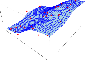
FIGURE 2.1. The Advertising data set. The plot displays sales , in thousands of units, as a function of TV , radio , and newspaper budgets, in thousands of dollars, for 200 different markets. In each plot we show the simple least squares fit of sales to that variable, as described in Chapter 3. In other words, each blue line represents a simple model that can be used to predict sales using TV , radio , and newspaper , respectively.
그림 2.1. Advertising 데이터 세트. 플롯은 200개의 서로 다른 시장들에 대해 수천 달러 단위의 TV, radio, 그리고 newspaper 예산들의 함수로서 수천 단위의 sales 를 표시합니다. 각 도표에서 우리는 3장에서 설명된 바와 같이 해당 변수에 대한 sales 의 단순 최소 제곱 적합(simple least squares fit)을 보여줍니다. 다시 말해, 각각의 파란색 선은 각각 TV, radio, 그리고 newspaper 를 사용하여 sales 를 예측하는 데 사용될 수 있는 단순한 모델을 나타냅니다.
Here f is some fixed but unknown function of $X_1, . . . , X_p$ , and ϵ is a random error term , which is independent of X and has mean zero.
여기서 f 는 어떤 고정되어 있지만 알려지지 않은 $X_1, \dots , X_p$ 의 함수이며, ϵ 은 무작위 오차 항(error term) 으로써 X 와 독립적이고 평균이 0입니다.
In this formulation, f represents the systematic information that X provides about Y .
이러한 공식화에서 f 는 X 가 Y 에 대해 제공하는 체계적인(systematic) 정보를 나타냅니다.
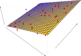
FIGURE 2.2. The Income data set. Left: The red dots are the observed values of income (in thousands of dollars) and years of education for 30 individuals. Right: The blue curve represents the true underlying relationship between income and years of education , which is generally unknown (but is known in this case because the data were simulated). The black lines represent the error associated with each observation. Note that some errors are positive (if an observation lies above the blue curve) and some are negative (if an observation lies below the curve). Overall, these errors have approximately mean zero.
그림 2.2. Income 데이터 세트. 좌측: 빨간색 점들은 30명의 개인들에 대한 income (수천 달러 단위)과 years of education 의 관측 값들입니다. 우측: 파란색 곡선은 일반적으로는 알려지지 않은(그러나 이 경우에는 데이터가 시뮬레이션되었기 때문에 알려진) income 과 years of education 간의 진정한 기저 관계를 나타냅니다. 검은색 선들은 각 관측치와 관련된 오차를 나타냅니다. 일부 오차들은 (관측치가 파란색 곡선 위에 위치한다면) 양수이고 일부는 (관측치가 곡선 아래에 위치한다면) 음수임에 주의하십시오. 전반적으로 이러한 오차들은 대략적으로 평균이 0입니다.
As another example, consider the left-hand panel of Figure 2.2, a plot of income versus years of education for 30 individuals in the Income data set.
또 다른 예로, Income 데이터 세트에서 30명의 개인들에 대한 years of education 대 income 도표인 그림 2.2의 좌측 패널을 고려해 보십시오.
The plot suggests that one might be able to predict income using years of education.
해당 도표는 years of education 을 사용하여 income 을 예측할 수 있을지도 모름을 시사합니다.
However, the function f that connects the input variable to the output variable is in general unknown.
그러나 입력 변수를 출력 변수와 연결하는 함수 f 는 일반적으로 알려져 있지 않습니다.
In this situation one must estimate f based on the observed points.
이 상황에서는 관측된 점들에 기초하여 f 를 추정해야 합니다.
Since Income is a simulated data set, f is known and is shown by the blue curve in the right-hand panel of Figure 2.2.
Income 이 시뮬레이션된 데이터 세트이므로 f 는 알려져 있으며, 그것은 그림 2.2의 우측 패널에 있는 파란색 곡선으로 보입니다.
The vertical lines represent the error terms ϵ .
수직선들은 오차 항들 ϵ 을 나타냅니다.
We note that some of the 30 observations lie above the blue curve and some lie below it; overall, the errors have approximately mean zero.
우리는 30개의 관측치 중 일부가 파란색 곡선 위에 위치하고 일부는 그 밑에 위치함에 주목합니다; 전반적으로 그 오차들은 대략 0의 평균을 갖습니다.
In general, the function f may involve more than one input variable.
일반적으로, 함수 f 는 둘 이상의 입력 변수를 포함할 수 있습니다.
In Figure 2.3 we plot income as a function of years of education and seniority .
그림 2.3에서 우리는 years of education 과 seniority 의 함수로서 income 을 그렸습니다.
Here f is a two-dimensional surface that must be estimated based on the observed data.
여기서 f 는 관측된 데이터에 기초하여 추정되어야만 하는 2차원 표면입니다.
In essence, statistical learning refers to a set of approaches for estimating f .
본질적으로, 통계적 학습은 f 를 추정하기 위한 일련의 접근법들을 나타냅니다.
In this chapter we outline some of the key theoretical concepts that arise in estimating f , as well as tools for evaluating the estimates obtained.
이 장에서 우리는 얻어진 추정치들을 평가하기 위한 도구들뿐만 아니라 f 를 추정하는 데 발생하는 주요 이론적 개념들의 일부를 개괄합니다.
2.1.1 Why Estimate f ? (왜 f를 추정해야 하는가?)
새로운 데이터 포인트에 대해 출력값을 예측하기 위한 예측(Prediction) 중심의 이유와,
각 입력 변수가 출력 변수에 미치는 영향을 분석하기 위한 추론(Inference) 중심의 이유를 배웁니다.
2.1.2 How Do We Estimate f ? (어떻게 f를 추정하는가?)
학습 데이터(Training Data)를 활용하여 가장 적합한 함수 $f$를 수학적으로 구성하는 접근 방식을 소개합니다.
파라미터 모델(Parametric)과 비-파라미터 모델(Non-Parametric)의 근본적인 차이점과 작동 원리를 다룹니다.
2.1.3 The Trade-Off Between Prediction Accuracy and Model Interpretability (예측 정확도와 모델 해석력 간의 트레이드오프)
모델이 유연하고 강력해질수록 내부 구조가 복잡해지며 원인 분석과 해석이 크게 어려워지는 블랙박스 구조 현상을 다룹니다.
분석의 근본 목적(높은 정확성 vs 구체적인 원인 규명 필요성)에 따라 유연성 수준을 결정하는 능력을 기릅니다.
2.1.4 Supervised Versus Unsupervised Learning (지도 학습과 비지도 학습)
예측 대상이 되는 정답(Label/Response)이 주어지는 환경에서의 지도 학습과 구조적인 특징만을 파악하는 비지도 학습의 차이를 짚어봅니다.
결과적으로 지도-비지도 중간의 성격을 지닌 반지도 학습(Semi-Supervised) 개념도 짧게 소개됩니다.
2.1.5 Regression Versus Classification Problems (회귀 문제와 분류 문제)
반응 변수가 수치적으로 연속형인 회귀(Regression) 상황과 질적으로 나뉘는 이산형인 분류(Classification) 상황을 정의합니다.
각 문제 유형에 알맞은 알고리즘과 평가지표 체계가 본질적으로 달라져야 함을 설명합니다.
2.1.1 Why Estimate f ? (왜 f를 추정해야 하는가?)
새로운 데이터 포인트에 대해 출력값을 예측하기 위한 예측(Prediction) 중심의 이유와, 각 입력 변수가 출력 변수에 미치는 영향을 분석하기 위한 추론(Inference) 중심의 이유를 배웁니다.
2.1.2 How Do We Estimate f ? (어떻게 f를 추정하는가?)
학습 데이터(Training Data)를 활용하여 가장 적합한 함수 $f$를 수학적으로 구성하는 접근 방식을 소개합니다. 파라미터 모델(Parametric)과 비-파라미터 모델(Non-Parametric)의 근본적인 차이점과 작동 원리를 다룹니다.
2.1.3 The Trade-Off Between Prediction Accuracy and Model Interpretability (예측 정확도와 모델 해석력 간의 트레이드오프)
모델이 유연하고 강력해질수록 내부 구조가 복잡해지며 원인 분석과 해석이 크게 어려워지는 블랙박스 구조 현상을 다룹니다. 분석의 근본 목적(높은 정확성 vs 구체적인 원인 규명 필요성)에 따라 유연성 수준을 결정하는 능력을 기릅니다.
2.1.4 Supervised Versus Unsupervised Learning (지도 학습과 비지도 학습)
예측 대상이 되는 정답(Label/Response)이 주어지는 환경에서의 지도 학습과 구조적인 특징만을 파악하는 비지도 학습의 차이를 짚어봅니다. 결과적으로 지도-비지도 중간의 성격을 지닌 반지도 학습(Semi-Supervised) 개념도 짧게 소개됩니다.
2.1.5 Regression Versus Classification Problems (회귀 문제와 분류 문제)
반응 변수가 수치적으로 연속형인 회귀(Regression) 상황과 질적으로 나뉘는 이산형인 분류(Classification) 상황을 정의합니다. 각 문제 유형에 알맞은 알고리즘과 평가지표 체계가 본질적으로 달라져야 함을 설명합니다.
Sub-Chapters (하위 목차)
| < 2. Statistical Learning | 2.1.1 Why Estimate F > |